Implicit Q-Learning with TorchRL

This tutorial demonstrates how to use a Minari dataset in conjunction with TorchRL to train an offline RL agent. We use Implicit Q-Learning to learn how to control a 24-dof hand to manipulate a pen, learning from a dataset of just 25 human demonstrations. We will cover:

• Working with Gymnasium environments in TorchRL.

• Creating a replay buffer from a Minari dataset.

• The basics of Implicit Q-Learning (IQL).

• Setting up an IQL training loop and training an agent.

The IQL implementation here is based in part on the offline IQL example script in TorchRL. Other offline RL algorithms are available there as well.

Pre-requisites

This tutorial currently requires a recent nightly build of TorchRL:

! pip install "torchrl-nightly>=2023.12.30"
! pip install matplotlib minari gymnasium-robotics

Note: If you run into conflicts with PyTorch when installing it, you may have to first install PyTorch nightly. Remember to add the “-U” flag to upgrade torch if it’s already installed.

To confirm that everything is installed properly we import the required modules:

import warnings
import matplotlib.pyplot as plt
import numpy as np
import gymnasium
import torch
import torchrl

seed = 42
torch.manual_seed(seed)
np.random.seed(seed)
warnings.simplefilter("ignore")

For headless environments

If you are in a headless environment (e.g. a Google Colab notebook), you will also need to install a virtual display. First, install the prerequisites:

! sudo apt-get update
! sudo apt-get install -y python3-opengl
! apt install ffmpeg
! apt install xvfb
! pip install pyvirtualdisplay

Then restart the notebook kernel. Once the pre-requisites are installed you can start a virtual display:

from pyvirtualdisplay import Display

virtual_display = Display(visible=0, size=(1400, 900))
virtual_display.start()

The Adroit Pen environment

from torchrl.envs.libs.gym import GymEnv
from torchrl.envs import DoubleToFloat, TransformedEnv

We will be using the AdroitHandPen environment from Gymnasium-Robotics. TorchRL is designed to be agnostic to different frameworks, so instead of working with a Gymnasium environment directly we load it using the GymEnv wrapper:

env_id = "AdroitHandPen-v1"
example_env = GymEnv(env_id, from_pixels=True, pixels_only=False)
example_env.set_seed(seed)

GymEnv provides the usual methods such as env.step() and env.reset(). However, instead of returning a tuple of step/reset data, they return a TensorDict. A tensordict is essentially a dictionary of tensors whose first axis (the batch dimension) has the same size, and share some other properties like the device they are on. The tensordict returned has fields for each type of step data (e.g. observations, actions, rewards):

tensordict = example_env.reset()
print(tensordict)

TensorDict(
    fields={
        done: Tensor(shape=torch.Size([1]), device=cpu, dtype=torch.bool, is_shared=False),
        observation: Tensor(shape=torch.Size([45]), device=cpu, dtype=torch.float64, is_shared=False),
        pixels: Tensor(shape=torch.Size([480, 480, 3]), device=cpu, dtype=torch.uint8, is_shared=False),
        terminated: Tensor(shape=torch.Size([1]), device=cpu, dtype=torch.bool, is_shared=False),
        truncated: Tensor(shape=torch.Size([1]), device=cpu, dtype=torch.bool, is_shared=False)},
    batch_size=torch.Size([]),
    device=cpu,
    is_shared=False)

TorchRL also provides env.rollout() to step through a full episode and save the step data in a tensordict:

max_episode_steps = 1000
tensordict = example_env.rollout(max_steps=max_episode_steps, auto_cast_to_device=True)

We can compute the cumulative reward by summing tensordict['next', 'reward']:

print(f"Cumulative reward: {tensordict['next', 'reward'].sum():.2f}")

Cumulative reward: 884.10

Because we specified from_pixels=True when initialising the environment, the pixels field of the tensordict is populated with image data. Here’s the first frame of that episode:

plt.imshow(tensordict["pixels"][0].numpy());

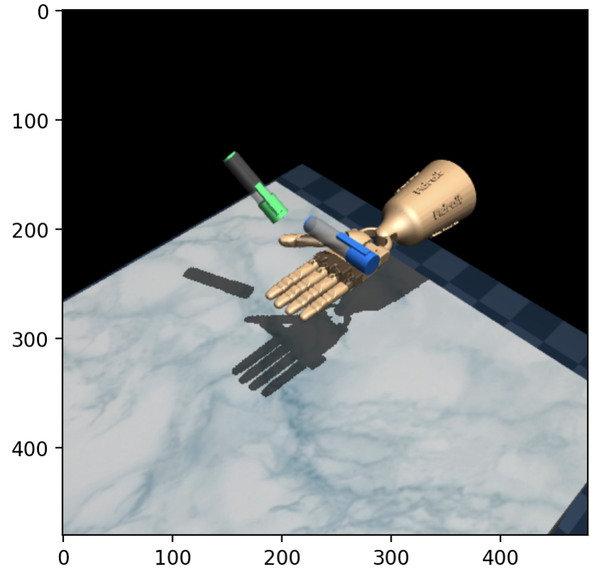
The aim of the Adroit Pen task is to control the 24-dof hand to manipulate the blue pen from the initial configuration (shown above) to the goal configuration (green pen). There is a shaped dense reward which quantifies how close the pen is to the target configuration, which is randomised at the start of each episode.

To use this environment for training, we need to perform some pre-processing transforms on the step data returned. We transform the base environment with DoubleToFloat(), which converts all doubles in the observations to floats:

device = torch.device("cuda" if torch.cuda.is_available() else "cpu")

base_env = GymEnv(env_id, device=device)
env = TransformedEnv(base_env, DoubleToFloat())
env.set_seed(seed)

Building a replay buffer

The Minari dataset we will be using is pen-human-v1, which consists of 25 human demonstrations. We can create a replay buffer using MinariExperienceReplay():

from torchrl.data.datasets.minari_data import MinariExperienceReplay
from torchrl.data.replay_buffers import SamplerWithoutReplacement

dataset_id = "pen-human-v1"
batch_size = 256

replay_buffer = MinariExperienceReplay(
    dataset_id,
    split_trajs=False,
    batch_size=batch_size,
    sampler=SamplerWithoutReplacement(),
    transform=DoubleToFloat(),
)

Note: We add the transform DoubleToFloat() so that the step data is consistent with our environment.

On the first run, the dataset will be downloaded from Farama servers and stored in the local cache directory (e.g. ~/.cache/torchrl/minari/). Once the dataset is loaded we can iterate over the replay buffer or use replay_buffer.sample() to load batches of transitions.

Implicit Q-Learning

For completeness, we give a quick overview of Implicit Q-Learning (IQL) and how it tries to tackle some of the challenges of offline RL. Those who are familiar with IQL or are only interested in the practical implementation can skip to the next section: Defining the model.

The main challenge in offline RL is distribution shift: Function approximators (e.g. for the Q-function) are trained on one distribution of data, the offline dataset, but are evaluated on another distribution, that of the newly trained policy. When evaluating state-action pairs well outside of the original distribution, they may extrapolate poorly, resulting in a policy that performs well on the dataset but poorly in practice. To make this more precise, consider an offline dataset \(\mathcal{D} = \{(s_t, a_t, r_t, s_{t+1}), \dots\}\). A standard starting point for offline RL algorithms is minimising the temporal difference error, by optimizing the objective

\[L_{\rm TD}(\theta) = \mathbb{E}_{(s, a, s') \sim \mathcal{D}} \left[ \left( r(s, a) + \gamma \max_{a'} Q_{\hat{\theta}}(s', a') - Q_\theta(s, a) \right)^2 \right]\]

Expectiles of an example conditional distribution \(y \sim m_\tau(s)\). For \(\tau = 0.5\) the expectile is the mean while for \(\tau \approx 1\) it approximates the maximum of the distribution (Kostrikov et al 2021).

where \(Q_{\hat{\theta}}\) is a target network, a lagged copy of \(Q_{\theta}\). Using the Q-function, one can then define a policy by \(\pi(s) \equiv \arg\max_a Q_\theta(s, a)\). However, this objective \(L_{\rm TD}\) requires evaluating the value of next actions \(a'\) that may not be in the dataset. If \(Q_{\hat{\theta}}(s', a')\) overestimates the value of the state-action \((s', a')\), the resulting arg-max policy may be overconfident. It is therefore important to limit overestimation of the values of out-of-distribution actions.

Implicit Q-Learning attempts to avoid this issue by never querying out-of-distribution state-action values \(Q(s', a')\). Instead of arg-maxing over \(Q(s', a')\), IQL introduces a value function \(V_\psi(s)\) which estimates the expectile of the state value function, an estimate of the maximum Q-value over actions that are in the support of the dataset distribution. We can fit \(V_\psi(s)\) using the objective

\[L_V(\psi) = \mathbb{E}_{(s, a) \sim \mathcal{D}} \left[ L_2^\tau (Q_{\hat{\theta}}(s, a) - V_\psi(s)) \right]\]

where \(L_2^\tau(u) \equiv \left| \tau - \mathbb{1}(u < 0) \right| u^2\). This specific choice of objective fits \(V_\psi(s)\) to the expectile of the state-action value function with respect to the dataset action distribution. See the figure to the right for an example of some expectiles for different values of \(\tau\).

We then use \(V_\psi(s)\) to update the Q-function:

\[L_Q(\theta) = \mathbb{E}_{(s, a, s') \sim \mathcal{D}} \left[ \left( r(s, a) + \gamma V_\psi(s') - Q_\theta(s, a) \right)^2 \right].\]

This is the same as the original TD error objective \(L_{\rm TD}(\theta)\), except we use \(V_\psi(s')\) instead of trying to maximise \(Q(s', a')\). Once trained, this provides us with a Q-function which implicitly defines the policy. To extract the explicit policy, IQL uses advantage-weighted behavioural cloning:

\[L_\pi(\phi) = \mathbb{E}_{(s, a) \sim \mathcal{D}} \left[ e^{\beta(Q_{\hat{\theta}}(s, a) - V_\psi(s))} \log \pi_\phi(a | s) \right].\]

The hyperparameter \(\beta\) controls the influence of the advantage \(A(s, a) \equiv Q_{\hat{\theta}}(s, a) - V_\psi(s)\). For small values of \(\beta\), the objective \(L_\pi(\phi)\) behaves similarly to standard behavioral cloning, while for larger values, it attempts to recover the maximum of the Q-function.

In summary, IQL defines the following networks:

• A state value function \(V_\psi(s)\) that quantifies the value of the best action within the support of the dataset.

• A state-action value function \(Q_\theta(s, a)\) (and a target network \(Q_{\hat{\theta}}(s, a)\)).

• A policy \(\pi_\phi(a | s)\).

We can update all of these networks together by optimizing the total objective \(\ell = L_V(\psi) + L_Q(\theta) + L_\pi(\phi)\) using gradient descent.

Note: The IQL implementation here is designed to be simple, rather than a benchmarkable implementation. For an implementation that accurately reproduces benchmark scores, see e.g. CORL.

Defining the model

from tensordict.nn import TensorDictModule
from tensordict.nn.distributions import NormalParamExtractor
from torchrl.envs.utils import ExplorationType, set_exploration_type
from torchrl.modules import MLP, ProbabilisticActor, TanhNormal, ValueOperator
from torchrl.objectives import IQLLoss, SoftUpdate
from torchrl.trainers.helpers.models import ACTIVATIONS

We first initialise the value network \(V_\psi(s)\) which estimates the expectile of the value of a state \(s\) with respect to the distribution of actions in the dataset. TorchRL provides a MLP convenience class which we use to build a two layer Multi-Layer Perceptron. To plug this MLP into the rest of the network, we specify that the inputs are read from the "observation" and "action" keys of the input tensordict (and concatenated, by default), and the output of the MLP is written to the "state_value" key:

hidden_sizes = [128, 128]
activation_fn = ACTIVATIONS["relu"]

# MLP network
value_net = MLP(
    num_cells=hidden_sizes,
    out_features=1,
    activation_class=activation_fn,
)

# Specify the keys to read/write from the tensordict
value_net = ValueOperator(
    in_keys=["observation"],
    out_keys=["state_value"],
    module=value_net,
)

We similarly initialise the action-value network \(Q_{\theta}(s, a)\),

q_net = MLP(
    num_cells=hidden_sizes,
    out_features=1,
    activation_class=activation_fn,
)

qvalue = ValueOperator(
    in_keys=["observation", "action"],
    out_keys=["state_action_value"],
    module=q_net
)

Finally, we initialise the policy/actor \(\pi_\phi(a | s)\), representing the policy as a tanh-Normal distribution parameterised by location and scale. There are three steps in setting up the actor:

• Create an MLP network (as before).

• Map the MLP outputs to “location” and “scale” parameters, in particular so that the “scale” output is strictly positive.

• Wrap it with the ProbabilisticActor class, specifying the distribution type.

The ProbabilisticActor class provides a convenient way to work with RL policies. By passing it the action_spec of the environment, it will also ensure that the outputs respect the bounds of the action space – that every policy output is a valid action.

action_spec = env.action_spec

# Actor/policy MLP
actor_mlp = MLP(
    num_cells=hidden_sizes,
    out_features=2 * action_spec.shape[-1],
    activation_class=activation_fn,
)

# Map MLP output to location and scale parameters (the latter must be positive)
actor_extractor = NormalParamExtractor(scale_lb=0.1)
actor_net = torch.nn.Sequential(actor_mlp, actor_extractor)

# Specify tensordict inputs and outputs
actor_module = TensorDictModule(
    actor_net,
    in_keys=["observation"],
    out_keys=["loc", "scale"]
)

# Use ProbabilisticActor to map it to the correct action space
actor = ProbabilisticActor(
    module=actor_module,
    in_keys=["loc", "scale"],
    spec=action_spec,
    distribution_class=TanhNormal,
    distribution_kwargs={
        "min": action_spec.space.low,
        "max": action_spec.space.high,
        "tanh_loc": False,
    },
    default_interaction_type=ExplorationType.MODE,
)

For convenience, we gather the actor and value functions into a single “model”:

model = torch.nn.ModuleList([actor, qvalue, value_net]).to(device)

Under the hood, MLP() uses LazyLinear layers, whose shape is inferred during the first pass. Later methods need a fixed shape, so we forward some random data through the network to initialise the Lazy modules:

with torch.no_grad(), set_exploration_type(ExplorationType.RANDOM):
    tensordict = env.reset().to(device)

    for net in model:
        net(tensordict)

Loss and optimizer

The explicit details of the Implicit Q-Learning losses are captured by TorchRL’s IQLLoss module:

loss_module = IQLLoss(
    model[0],
    model[1],
    value_network=model[2],
    loss_function="l2",
    temperature=3,
    expectile=0.7,
)
loss_module.make_value_estimator(gamma=0.99)

IQL uses “soft updates” for the target network \(Q_{\hat{\theta}}(s, a)\). The target network parameters are slowly updated in the direction of \(Q_{\theta}(s, a)\) at each iteration via Polyak averaging \(\hat{\theta} \leftarrow \tau \,\theta + (1 - \tau) \, \hat{\theta}\),

target_net_updater = SoftUpdate(loss_module, tau=0.005)

We optimize all of the networks using Adam:

optimizer = torch.optim.Adam(loss_module.parameters(), lr=0.0003)

Training

To demonstrate training, we run IQL for 50,000 iterations. During training, we will evaluate the policy every 1000 iterations. But note that this is for evaluation purposes only. Unlike online RL, we do not collect new data during training.

@torch.no_grad()
def evaluate_policy(env, policy, num_eval_episodes=20):
    """Calculate the mean cumulative reward over multiple episodes."""
    episode_rewards = []

    for _ in range(num_eval_episodes):
        eval_td = env.rollout(max_steps=max_episode_steps, policy=policy, auto_cast_to_device=True)
        episode_rewards.append(eval_td["next", "reward"].sum().item())

    return np.mean(episode_rewards)

The training loop is essentially the standard PyTorch gradient descent loop:

1. Sample a batch of transitions from the dataset \(\mathcal{D}\).

2. Compute the loss \(\ell = L_V(\psi) + L_Q(\theta) + L_\pi(\phi)\).

3. Backpropagate the gradients and update the networks, including the target Q-network.

from tqdm.auto import tqdm

iterations = 10_000  # Set to 50_000 to reproduce the results below
eval_interval = 1_000

loss_logs = []
eval_reward_logs = []
pbar = tqdm(range(iterations))

for i in pbar:
    # 1) Sample data from the dataset
    data = replay_buffer.sample()

    # 2) Compute loss l = L_V + L_Q + L_pi
    loss_dict = loss_module(data.to(device))
    loss = loss_dict["loss_value"] + loss_dict["loss_qvalue"] + loss_dict["loss_actor"]
    loss_logs.append(loss.item())

    # 3) Backpropagate the gradients
    optimizer.zero_grad()
    loss.backward()
    optimizer.step()  # Update V(s), Q(a, s), pi(a|s)
    target_net_updater.step()  # Update the target Q-network

    # Evaluate the policy
    if i % eval_interval == 0:
        eval_reward_logs.append(evaluate_policy(env, model[0]))
        pbar.set_description(
            f"Loss: {loss_logs[-1]:.1f}, Avg return: {eval_reward_logs[-1]:.1f}"
        )

pbar.close()

We can plot the loss and episodic return:

fig, axes = plt.subplots(nrows=1, ncols=2, figsize=(7, 3))
axes[0].plot(loss_logs)
axes[0].set_title("Loss")
axes[0].set_xlabel("iterations")
axes[1].plot(eval_interval * np.arange(len(eval_reward_logs)), eval_reward_logs)
axes[1].set_title("Cumulative reward")
axes[1].set_xlabel("iterations")
fig.tight_layout()
plt.show()

Results

from IPython.display import HTML
from gymnasium.utils.save_video import save_video
from base64 import b64encode

Evaluated over 100 episodes, the final performance is:

final_score = evaluate_policy(env, model[0], num_eval_episodes=100)
print(f"Cumulative reward (averaged over 100 episodes): {final_score:.2f}")

Cumulative reward (averaged over 100 episodes): 1872.69

To visualise its performance, we can roll out a single episode and render the result as a video:

viewer_env = TransformedEnv(
    GymEnv(env_id, from_pixels=True, pixels_only=False),
    DoubleToFloat()
)
viewer_env.set_seed(seed)

tensordict = viewer_env.rollout(max_steps=max_episode_steps, policy=model[0], auto_cast_to_device=True)
print(f"Cumulative reward: {tensordict['next', 'reward'].sum():.2f}")

frames = list(tensordict["pixels"].numpy())
save_video(frames, video_folder="results_video", fps=30)

# Display the video. Embedding is necessary for Google Colab etc
mp4 = open("results_video/rl-video-episode-0.mp4", "rb").read()
data_url = "data:video/mp4;base64," + b64encode(mp4).decode()
HTML("""
<video controls style='margin: auto; display: block'>
    <source src='%s' type='video/mp4'>
</video>
""" % data_url)

Here are some examples of our trained agent:

The performance varies quite a bit from episode to episode, but overall it’s decent considering there are only 25 demonstrations in the original dataset! To improve performance, you could try tuning the hyperparameters, such as the inverse temperature \(\beta\) and the expectile \(\tau\), or use a larger dataset such as pen-expert-v1 which has around 5000 episodes.